1. Axial Force Diagram
Click ![]() , to see the Axial Force Diagram. You may take the picture below.
, to see the Axial Force Diagram. You may take the picture below.
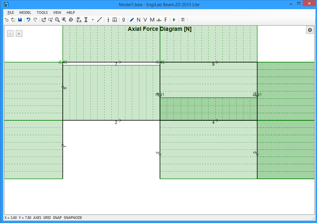
The Axial Force Diagram is out of Scale. Click the "Zoom All" button ![]() to automatically scale the Diagram.
to automatically scale the Diagram.
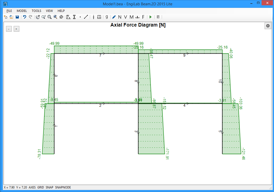
Now the result should look like this, which is much better.
2. Shear Force Diagram
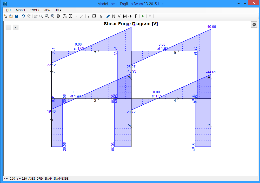
Click ![]() , to see the Shear Force Diagram. If the Shear Force Diagram is out of Scale, Click the "Zoom All" button
, to see the Shear Force Diagram. If the Shear Force Diagram is out of Scale, Click the "Zoom All" button ![]() to automatically scale the Diagram. You should take the following picture.
to automatically scale the Diagram. You should take the following picture.
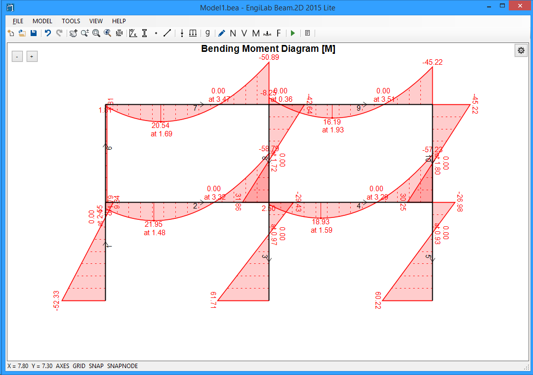
3. Bending Moment Diagram
Click ![]() , to see the Bending Moment Diagram. If the Bending Moment Diagram is out of Scale, Click the "Zoom All" button
, to see the Bending Moment Diagram. If the Bending Moment Diagram is out of Scale, Click the "Zoom All" button ![]() to automatically scale the Diagram. You should take the following picture.
to automatically scale the Diagram. You should take the following picture.
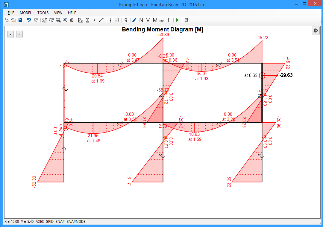
Note that if you move the pointer over an Element, you can read the corresponding value of the Diagram, as shown below for the Bending Moment Diagram case. This happens for all Diagrams and also for the Deformation and the Free Body Diagram.
4. Deformation
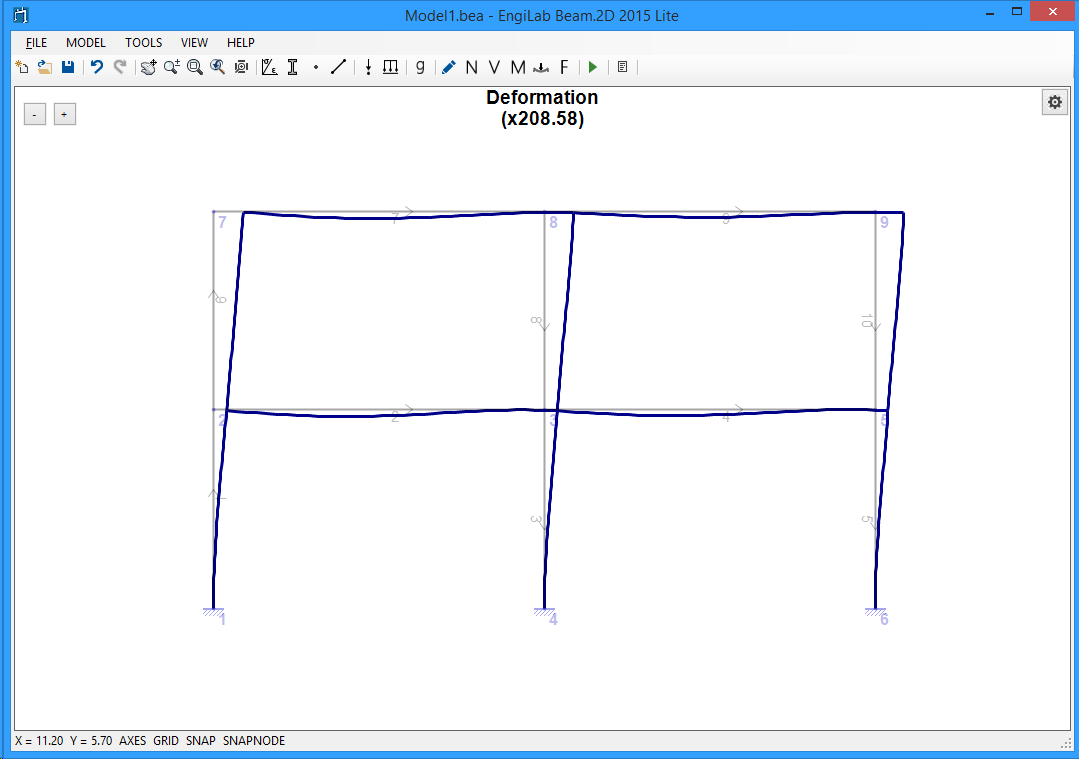
Click ![]() , to see the Model Deformation. If the Deformation is out of Scale, Click the "Zoom All" button to automatically scale it. You should take the following picture. The program reports also the Deformation magnification, in our example x208.58.
, to see the Model Deformation. If the Deformation is out of Scale, Click the "Zoom All" button to automatically scale it. You should take the following picture. The program reports also the Deformation magnification, in our example x208.58.
You can adjust scaling yourself by using the +/- buttons at the top left of the picture. If you click the "+" button a few times, you may get a picture like the one below where the magnification factor is now x521.46.
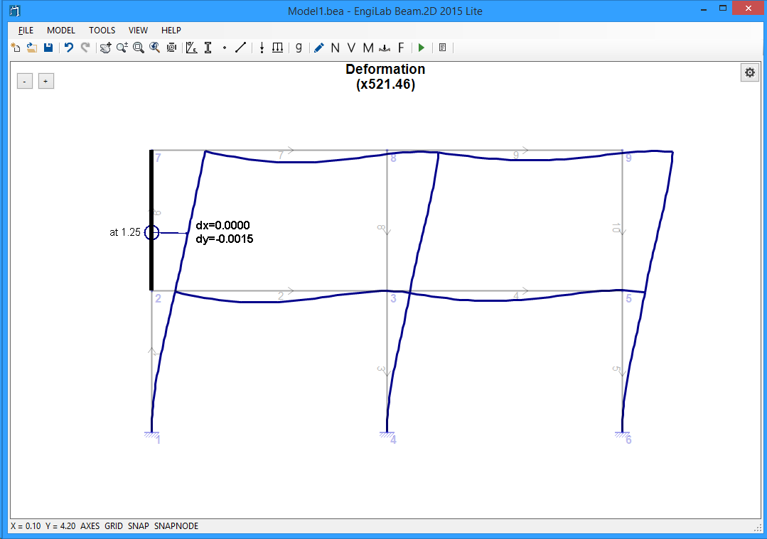
See above that you can get the deformation values on screen, if the mouse pointer moves over an element.
IMPORTANT: The values that are given on screen are the x and y displacements of the corresponding point of each element in Local Element Axes. For example, in the picture below Element 6 goes upward, which means that the Element x-Axis is pointing upwards and the Element y-Axis is pointing to the left. The point at 1.25 from the Element start (Node 2) has a deformation dy=-0.0015 m towards the Element y-direction (that means 0.0015 m to the right of the picture), which is equivalent to a deformation DX=0.0015 m in Global Axes (Global X-Axis points towards the right of the picture).
Note: EngiLab Frame.2D 2022 (v4.0) and later, shows the deformations in both Local Element Axes and Global Axes. See for example Example 2 - Step 11.
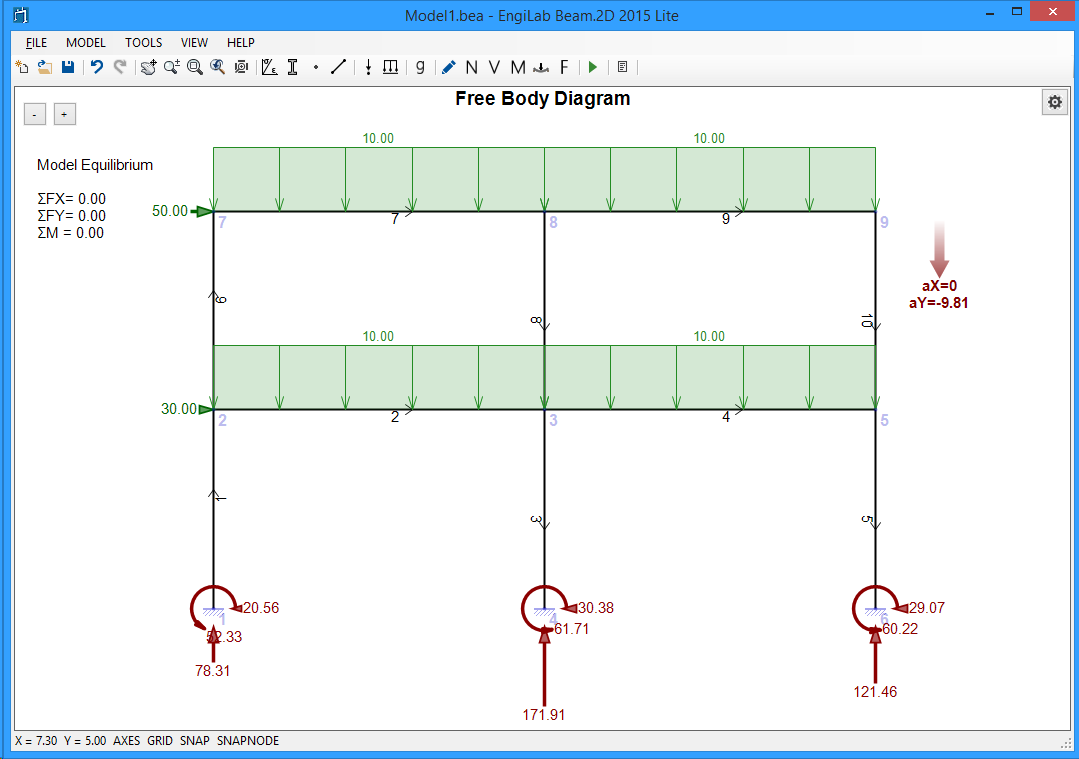
5. Free Body Diagram (F)
Click ![]() , to see the Free Body Diagram of the Model. The Free Body Diagram shows the support reactions on screen and also the calculations of the equilibrium of the Model.
, to see the Free Body Diagram of the Model. The Free Body Diagram shows the support reactions on screen and also the calculations of the equilibrium of the Model.
Note that if you move the pointer over an Element, you can read the corresponding N, V, M values, as shown below. The Element End Forces are also given on screen, for the specific Element and also the calculation of the equilibrium of the specific Element.
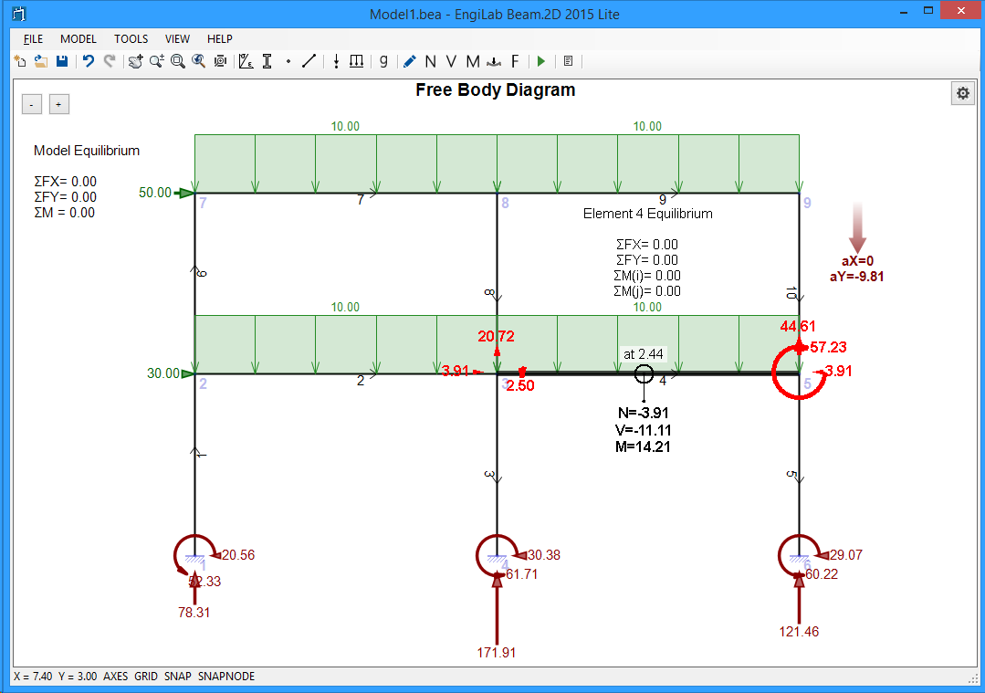
IMPORTANT: In the example above, we see the calculations of the equilibrium of Element 4 of the Model. All equilibrium calculations (ΣFX, ΣFY, ΣM(i), ΣM(j)) are zero, otherwise there would be a problem in our Model or in the analysis results. One may want to calculate the equilibrium of Element 4 on his own, for example the value ΣFY. There is an external uniform load with value 10, acting along Element 4 (Length = 5 m), which gives an external load of 10*5=50 kN acting towards -Y direction (downwards). The Element end forces sum up to 20.72+44.61=65.33 kN, towards Y direction (upwards). So why is there this difference of 65.33-50 = 15.33 kN? Is there a problem with the calculations?
The answer is NO. This is because of the self-weight of Element 4 which results to an additional uniform load (which is not shown on screen) acting towards -Y direction. Let's calculate this additional load:
Self weight of Element 5 (in kN) = Mass * Acceleration = Volume * Density * Acceleration = Area * Length * Density * Acceleration = 0.125 * 5 * 2.5 * 9.81 = 15.33 kN.
So, the correct equilibrium calculation should be: ΣFY = 50 + 15.33 - 65.33 = 0.00 kN which is reported by the program for Element 4.